Generalized Estimating Equations

Presentation Slides

Introduction

Generalized Estimating Equations (GEE) is a statistical methodology in a class of models that model the mean of an outcome as function of predictor variables commonly used to analyze correlated data in various fields that use panel or longitudinal data, including epidemiology, social sciences, and clinical trials (S. McCulloch C. 2008). The method was first introduced by Liang and Zeger in a paper in 1986 (Liang and Zeger 1986). The method uses a quasilikelihood approach and yields population averaged estimates of parameters (M. Wang 2014).

Analysis of longitudinal data has inherent problems with independence involving multiple observations for the same individual in clinical data studies. Liang and Zeger even referred to time dependence on multiple observations of an individual as a nuisance due to correlation issues (Liang and Zeger 1986). Another challenge for use of longitudinal data is the need for more complex statistical models to deal with the lack of independence in observations that could include multidimensional levels of integration, and the software is often not available (Donald and Robert 2006). The use of GEE mitigates these challenges with use of longitudinal data.

GEE extends the generalized linear model framework to account for within-cluster correlations, such as repeated observations or clustered data (Shao et al. 2023). GEE is used to model the marginal mean response while allowing for flexible correlation structures among observations within the same group or cluster. GEE estimates population-average effects by specifying a working correlation structure such as independence or exchangeable structures (Shao et al. 2023). GEE also implements an estimating equation approach to iteratively update the parameter estimates.

This methodology provides reliable and robust estimates, even when the correlation structure is mis-specified (M. Wang 2014). GEE is particularly useful for longitudinal or panel data analysis, as it allows for examination of all available data in the experiment and provides statistical inference for population-level ramifications (Lin and Perng 2011). Its ability to handle missing data makes GEE a great choice for analyzing correlated data, particularly in biostatistics or research settings without the use of intense statistical mathematics.

Methodology

Estimating Equations

Instead of maximizing the likelihood function, GEE employs a quasilikelihood estimating equation approach, as \(\beta\) estimates are based on the mean and variance of the population (D’Angelo et al. 2011). The estimating equations are derived based on the assumed correlation structure and the marginal mean model,not a specified distribution (D’Angelo et al. 2011). GEE models can be for continuous, binary or count outcomes for changes in population mean as a function of predictor variables.

Iterative Algorithm

In the GEE process, IRLS, iteratively reweighed least squares, is used for estimates of the dispersion parameter \(\alpha\) to determine new estimates for the \(\beta\) estimators or coefficients of predictor variables after using initial estimate until convergence of the estimators occurs. Once there is convergence and \(\beta\) estimators for each variable are known, then hypothesis testing, calculating confidence intervals for each of the estimators can be done and standard errors obtained (Donald and Robert 2006).

Software packages, such as ‘geepack’ package in R handle the iteration process. The iterative process works until there is convergence to stable estimates Liang and Zeger (1986).

Data Structure

GEE is designed for analyzing relationships between population means and correlated data, such as longitudinal or panel data in which the data is organized into clusters, where each cluster represents a group of related observations (epidemiology, social sciences, clinical trials, etc) (S. McCulloch C. 2008). The assumption of independent observations may not be accurate. A GEE analysis of a dataset with longitudinal data with repeated observations per individual will be shown using the respiratory dataset available through the ‘geepack’ package in R (Halekoh, Højsgaard, and Yan 2006).

Model Specification

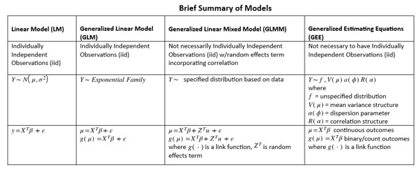
GEE is an extension of generalized linear models (GLM) and uses that framework to specify the relationship between the response variable and the regressor variables by adding the use of correlation structures to handle possible correlation in the data with population mean outcomes (Shao et al. 2023). The choice of the link function and the distribution of the response variable depends on the nature of the data (Gayen and Kumar 2018). Models can be created for population means for continuous, binary or count outcomes. The table below shows the extension of GEE from the LM, GLM,and GLMM and differences in assumptions.

Figure 1: Model Comparison and Summary (S. McCulloch C. 2008)

According the Liang and Zeger, the method of GEE, longitudinal data sets, are comprised of an outcome variable, \(y_{it}\), and $$p\times1$$ vector of covariates, \(x_{it}\), observed at times \[t=1,...,n_{it}\] for subjects \[i=1,...,K\] which arise often in applied sciences (Liang and Zeger 1986). For example, in health care study data, individual patients have followup visits to monitor a treatment plan and therefore have multiple observations for each patient. GEE is used for these kind of longitudinal datasets due to the use of correlation structures in its modeling design to account for the lack of independence in the repeated observations.

In Wang’s review of GEE method, a marginal model specifying a relationship between \(\mu_i\) and \(X_{ij}\) is given by the equation \(g(\mu_{ij})=X'_{ij} \beta\), where \(g\) is the link function and \(\beta\) is a vector of regression coefficients and then shows the mathematical calculations to get to the equation

\(U(\beta) = \sum_{i=1}^K {D_i}^{\prime} {V_i}^{-1}(Y_i-\mu_i)=0\)

that when solved will give estimates of \(\beta_i\) used in the generated models. In this equation \(D_i=\partial\mu_i/\partial\beta^{\prime}\) and \({V_i}^{-1}\) is the inverse of the variance-covariance matrix for \(Y_i\), \(V_i = \phi{A_i}^{1/2}R_i(a){A_i}^{1/2}\) , \(A_i\) is a diagonal matrix with elements that are known variance functions of \(\mu_{ij}\) times a scaling parameter \(\phi\), and \(R_i(a)\) is the correlation structure (M. Wang 2014). Since the equation used for solving for \(\beta\) depends only on the mean and variance, the estimates are referred to as quasilikelihood estimates and not based on the more complex statistical mathematics for determining maximum likelihood estimates as can be the case for GLMM (Donald and Robert 2006).

GEE employ a logistic regression model created using the ‘geepack’ package available in R, specifying a correlation structure (see the structure types in the paragraph below), family type of binomial for discrete outcomes and would yield model of

General mathematical formula for multivariate GEE modeling the population mean using the logit link function for binary outcomes: \[ g(\mu)= \text{logit}[P(y_\text{ij}=1)]=log\left(\dfrac{\pi_{ij}}{1-\pi_{ij}}\right)=\beta_0+Regressor1_{ij}\beta_1+Regressor2_{ij}\beta_2...+RegressorN\beta_{N-1} \]

that predicts average change in the log odds for population mean outcomes for each predictor variable (Statistics 2023).

The ‘geepack’ package in R uses the link and variance functions in the geeglm() function of identity for Gaussian, logit and \(\mu(1-\mu),\mu\in(0,1)\) for binomial, log and\(\mu,\mu>0\) for poisson, and log and \(\mu^2,\mu>0\) for gamma families (Halekoh, Højsgaard, and Yan 2006).

In order to have confidence intervals and hypothesis testing for the for the estimated regression coefficients, standard error must be calculated and can be found by taking the square root of the diagonal elements of \(V(\hat\beta)\) yielding two types of standard error, naive and robust (Donald and Robert 2006).

Correlation Structures

GEE allows for flexible modeling of the correlation structure within clusters. A working correlation structure is specified, which represents the assumed relationship among the correlated observations (Seals and Aban 2016). The correlation structures discussed in this paper are exchangeable, auto-regressive (AR1), unstructured, and independent.

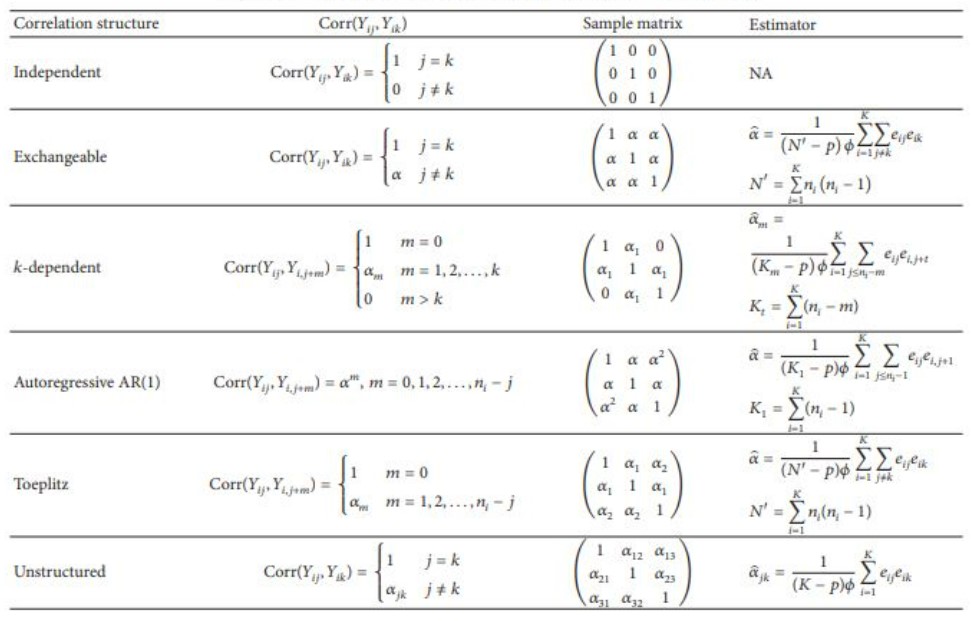
Figure 2: Correlation Structures Comparison Table (M. Wang 2014)

The independent correlation structure is used when the assumption between multiple repeated observations of a single individual is independent. Use of the exchange correlation structure is used when there is equality between times of observations. Auto-regressive (AR1) correlation structure is used when there are more than one set of equal time differences between repeated observations. And lastly, unstructured correlation structure is the most general and takes into account all the possible time intervals between repeated observations. Of course there are more choices for correlation structures, but these (4) structures are the structures used in the ‘geepack’ R package used in the subsequent examples.

If the correlation structure chosen for GEE is not correct, the predictor variables will still be estimated consistently, since the GEE method relies on the first moment, however the standard errors will be incorrect. This is considered a very attractive property of GEE models (Donald and Robert 2006). A possible remedy for choosing a correlation structure incorrectly is to use the ‘sandwich’ package in R that uses the Huber-White sandwich estimator to create an an approximation for the correlation Zeileis et al. (2019). By default, the ‘geepack’ package in R uses a sandwich estimator if the number of clusters is larger than 30, but has a built in options to use another variance estimator called the jackknife estimator, fully iterated or approximate, for cases where the number of clusters is less than 30 (as recommended by (Paik 1988)) (Halekoh, Højsgaard, and Yan 2006).

Correlation structure selection is determined through various methods and is not limited to the structures shown in the correlation table above. One valid method used to determine model selection has been proposed by Shults and Chaganty (L. Wang, Zhou, and Qu 2012) as to determine the structure based on the generalized error sum of squares given by the following equation: \[ ESS(\alpha,\beta) = \sum_{i=1}^{K}{(Y_i - \mu _i)}'{V_{i}}^{-1}(Y_i - \mu _i) \] In addition to the method by Shults and Chaganty, Wang discusses several other methods for correlation structure selection and cites many other methods available (M. Wang 2014).

Analysis and Results

Data and Visualisation

In this review of GEE, the ‘geepack’ package for R with a respiratory dataset included was used to showcase an example Yan (2002). The respiratory dataset included in the packet is an example of longitudinal or panel data as data is from a clinical study of 111 patients receiving treatment for a respiratory illness (Koch et al. 1990).

Figure 3: Respiratory Variable Summary

Variable	Description
center	a numeric vector
id	a numeric vector
treat	treatment or placebo
sex	male or female
age	in years at baseline
baseline	respiratory status at baseline
visit	id of visit
outcome	respiratory status at visit

Code

######## loading packages ########

library(tidyverse)
library(knitr)
library(geepack)
library(lme4)   # For fitting linear mixed models
library(glmmTMB)  # For fitting GLMMs with different distributions
library(ggeffects)
library(dplyr)
library(ggplot2)
library(furniture)

######## Load Data ########

data(respiratory)

displayData <- respiratory[respiratory$id < 4,]
displayData <- displayData[displayData$center == 2,]

######## Plot sample of data for visualization ########

ggplot(displayData, aes(x=visit, y=treat, color=factor(outcome))) +
  geom_point(size=5) +
  scale_x_continuous(breaks=c(1,2,3,4)) +
  scale_color_discrete("Respiratory Health",labels=c("Poor","Good")) +
  facet_grid(.~id) +
  labs(x = "Visit Number/Patient", y = "Treatent, 'A' = Treatment, 'P' = Placebo",title = "Figure 4: Respiratory Treatment Outcomes Over (4) Patient Visits")+
  theme_bw()

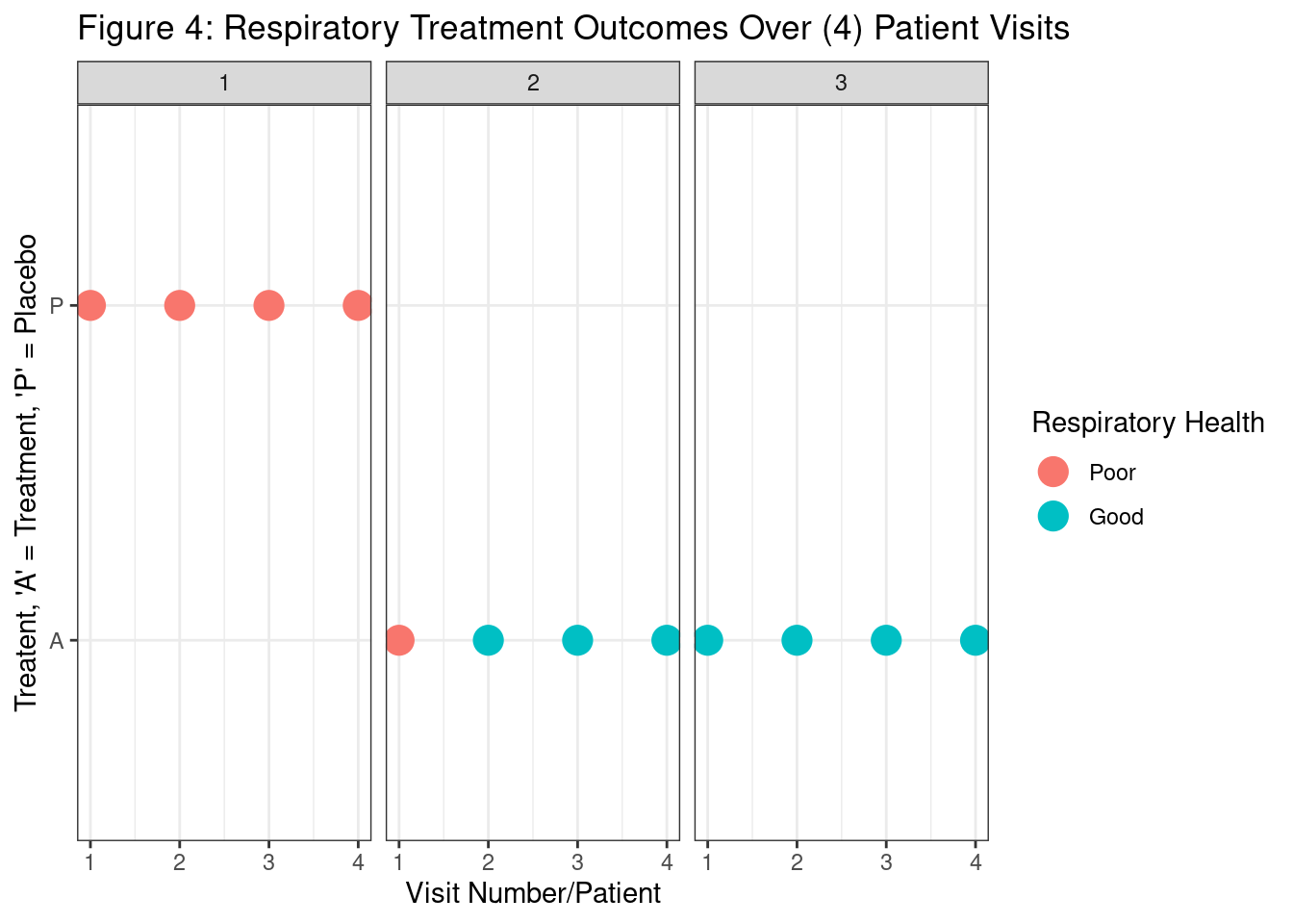
Figure 4, the above graphic, is displaying a small sample from the ‘respiratory’ data. The given data set is a study with longitudinal data of repeated measures with a binary outcome. There are four measures, or visits, performed on each individual. Each box with 1 through 4 on the x-axis represents a unique patient and their respective visits. The y-axis displays the treatment the patient is taking where P represents a placebo and A represents the actual treatment.

The points on the plot indicate the outcome of treatment and represent a patient’s respiratory status per visit where 1 indicates a “good” respiratory status and 0 indicates a “poor” respiratory status. Note that this graphic is a truncated form of the complete dataset and excludes both a treatment center and 52 other patients (Schwartz S 2023).

Code

###### Data transformation for "wide" data [record per visit] #######
resp_transformed <- respiratory %>% 
  tidyr::spread(key = visit,
                value = outcome,
                sep = "_") %>%
  dplyr::arrange(id) %>% 
  dplyr::select(id, center, 
                sex, age, treat, 
                baseline, starts_with("visit"))

‘resp_transformed’ is a data frame that has been transformed based on the original data set. This transformation manipulates the data such that there is one line per participant in the data. This method will allow for analyzing the metrics between repeated observations (Schwartz S 2023).

Code

###### Table of data breakdown - respiratory outcome over time #######
resp_transformed %>% 
  dplyr::group_by(treat) %>% 
  furniture::table1("Visit One" = visit_1, 
                    "Visit Two" = visit_2, 
                    "Visit Three" = visit_3, 
                    "Visit Four" = visit_4, 
                    caption = "Figure 5: 'Good' Respiratory Outcome Over Time",
                    output = "markdown",
                    na.rm = FALSE,
                    total = TRUE,
                    test = TRUE)

Figure 5: ‘Good’ Respiratory Outcome Over Time

	Total	A	P	P-Value
	n = 111	n = 54	n = 57
Visit One				0.038
	0.6 (0.5)	0.7 (0.5)	0.5 (0.5)
Visit Two				<.001
	0.5 (0.5)	0.7 (0.5)	0.4 (0.5)
Visit Three				0.004
	0.6 (0.5)	0.7 (0.5)	0.5 (0.5)
Visit Four				0.07
	0.5 (0.5)	0.6 (0.5)	0.4 (0.5)

Figure 5 “‘Good’ Respiratory Outcome Over Time” shows a breakdown of visits and the corresponding statistics for patients with a ‘good’ outcome. N is the total number of patients in the study, ‘A’ represents the treatment, and ‘P’ represents the placebo (Schwartz S 2023).

Code

###### Graph of Number of Visits with Poor Outcome #######
resp_transformed %>% 
  dplyr::mutate(n_good = furniture::rowsums(visit_1 == "0", 
                                            visit_2 == "0",
                                            visit_3 == "0",
                                            visit_4 == "0")) %>% 
  ggplot(aes(x = age,
             y = n_good)) +
  geom_count() +
  geom_smooth() +
  theme_bw() +
  labs(x = "Age in Years",
       y = "Number of Visits out of Four, with 'Poor' Respiration",
       title = "Figure 6: 'Poor' Respiration Outcomes for Total Visits")

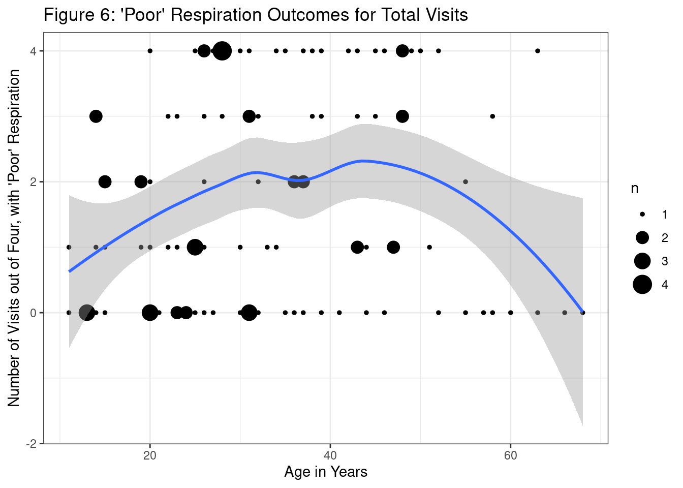
This visualization is focused on the age parameter in terms of outcome per visit. Based on age for the x-axis, it’s displaying whether respective patients had a ‘poor’ outcome (or poor respiration status) as a number out of the four total visits. The larger circles indicate a higher number of poor outcomes in total, while the smaller circles indicate a smaller number of poor outcomes in total. This visual does not display patients who had all ‘good’ outcomes (Schwartz S 2023).

Code

###### Correlation between repeated observations #######
resp_transformed %>% 
  dplyr::select(starts_with("visit")) %>% 
  dplyr::mutate_all(function(x) x == "1") %>% 
  cor() %>% 
  corrplot::corrplot(title = "Figure 7: Correlation Matrix for Repeated Visits",
                     mar=c(0,0,2,0))

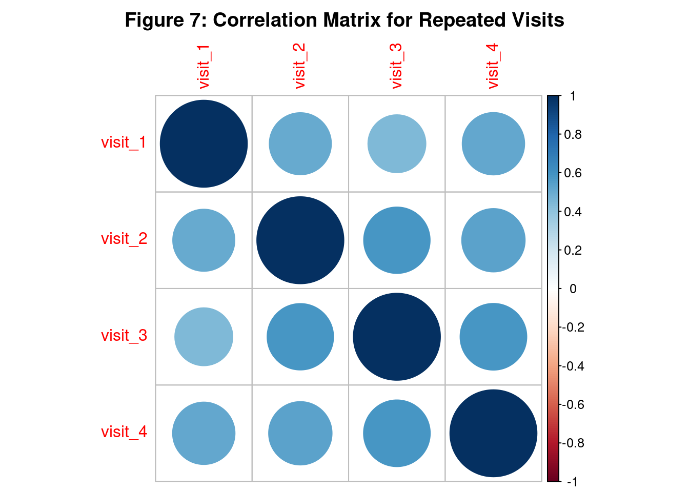
The preceding graphic, figure 7, shows the correlation matrix between repeated observations. It’s noted that there is a medium to high correlation between the observations. This is showing the necessity for a statistical model that can account for these levels of correlation between the observations (Schwartz S 2023).

Statistical Modeling

GEE Model(s)

GEE models focus on the mean of the correlated observations that are within groups and don’t focus on the distribution of the full data of the population (Halekoh, Højsgaard, and Yan 2006). GEE modeling requires parameters in the form of distribution of the response variable, the link function, the regressor variables, and the desired correlation structure. The various types of correlation structures were discussed in the previous methodology section; our example focuses on independent, exchangeable, unstructured, and auto-regressive order 1 correlation structures. The distribution selected for a model is based on the distribution of the response variable (Seals and Aban 2016) and may be a value such as binomial, Poisson, or Gaussian (Gayen and Kumar 2018). The link function parameter is contingent on the corresponding distribution where the distribution of the response variable dictates the model to be used (Agresti 2015).

The ‘geepack’ package in R was used to create four different models using the same geeglm() function and specifying different correlation structures as parameters within the function input. The binomial distribution is chosen for each model as well due to the binary response of a ‘poor’ or ‘good’ respiratory status. The canonical link function used for binary response data is ‘logit’ or logistic regression (Agresti 2015). This link function is inherently used in our models without direct specification.

1. GEE with Independent Correlation Structure

Code

# GEE with independent correlation structure
gee_independence <- geeglm(outcome ~ center + treat + age + baseline + sex, data=respiratory, id=id, 
                  family = binomial(), corstr="independence")
summary(gee_independence)

Call:
geeglm(formula = outcome ~ center + treat + age + baseline + 
    sex, family = binomial(), data = respiratory, id = id, corstr = "independence")

 Coefficients:
            Estimate  Std.err   Wald Pr(>|W|)    
(Intercept) -0.10346  0.88213  0.014 0.906634    
center       0.64949  0.35322  3.381 0.065952 .  
treatP      -1.26536  0.34668 13.322 0.000262 ***
age         -0.01876  0.01296  2.093 0.147974    
baseline     1.84572  0.34598 28.460 9.57e-08 ***
sexM        -0.13678  0.44025  0.097 0.756035    
---
Signif. codes:  0 '***' 0.001 '**' 0.01 '*' 0.05 '.' 0.1 ' ' 1

Correlation structure = independence 
Estimated Scale Parameters:

            Estimate Std.err
(Intercept)    1.002  0.1842
Number of clusters:   111  Maximum cluster size: 4 

(Halekoh, Højsgaard, and Yan 2006)

The GEE model summary with an independent correlation structure specified shows that there are no estimated correlation parameters. Referencing back to Figure 2, it’s noted that the estimator column for an independent correlation structure is empty. This is because the independent correlation structure is assuming there is no correlation between the observations within a cluster (Seals and Aban 2016).

2. GEE with Exchangeable Correlation Structure

Code

# GEE with exchangeable correlation structure
gee_exchangeable <- geeglm(outcome ~ center + treat + age + baseline + sex, data=respiratory, id=id, 
                  family = binomial(), corstr="exchangeable")
summary(gee_exchangeable)

Call:
geeglm(formula = outcome ~ center + treat + age + baseline + 
    sex, family = binomial(), data = respiratory, id = id, corstr = "exchangeable")

 Coefficients:
            Estimate Std.err  Wald Pr(>|W|)    
(Intercept)  -0.1035  0.8821  0.01  0.90663    
center        0.6495  0.3532  3.38  0.06595 .  
treatP       -1.2654  0.3467 13.32  0.00026 ***
age          -0.0188  0.0130  2.09  0.14797    
baseline      1.8457  0.3460 28.46  9.6e-08 ***
sexM         -0.1368  0.4402  0.10  0.75604    
---
Signif. codes:  0 '***' 0.001 '**' 0.01 '*' 0.05 '.' 0.1 ' ' 1

Correlation structure = exchangeable 
Estimated Scale Parameters:

            Estimate Std.err
(Intercept)        1   0.184
  Link = identity 

Estimated Correlation Parameters:
      Estimate Std.err
alpha    0.329  0.0838
Number of clusters:   111  Maximum cluster size: 4 

(Halekoh, Højsgaard, and Yan 2006)

The GEE model summary with an exchangeable correlation structure specified shows that there is one estimated correlation parameter. One again referencing back to Figure 2, it’s noted that the estimator parameter (\(\alpha\)) is contained in the working correlation structure. The \(\alpha\) value in the summary shows that there is an estimated 0.329 correlation value between visits for patients, or a 0.329 correlation value between observations in a cluster.

3. GEE with Unstructured Correlation Structure

Code

# GEE with unstructured correlation structure
gee_unstructured <- geeglm(outcome ~ center + treat + age + baseline + sex, data=respiratory, id=id, 
                  family = binomial(), corstr="unstructured")
summary(gee_unstructured)

Call:
geeglm(formula = outcome ~ center + treat + age + baseline + 
    sex, family = binomial(), data = respiratory, id = id, corstr = "unstructured")

 Coefficients:
            Estimate Std.err  Wald Pr(>|W|)    
(Intercept)  -0.1826  0.8685  0.04  0.83351    
center        0.6555  0.3513  3.48  0.06203 .  
treatP       -1.2455  0.3455 12.99  0.00031 ***
age          -0.0176  0.0129  1.87  0.17147    
baseline      1.8944  0.3441 30.31  3.7e-08 ***
sexM         -0.1144  0.4407  0.07  0.79528    
---
Signif. codes:  0 '***' 0.001 '**' 0.01 '*' 0.05 '.' 0.1 ' ' 1

Correlation structure = unstructured 
Estimated Scale Parameters:

            Estimate Std.err
(Intercept)     1.01   0.194
  Link = identity 

Estimated Correlation Parameters:
          Estimate Std.err
alpha.1:2    0.321   0.118
alpha.1:3    0.206   0.101
alpha.1:4    0.284   0.110
alpha.2:3    0.424   0.141
alpha.2:4    0.343   0.119
alpha.3:4    0.380   0.133
Number of clusters:   111  Maximum cluster size: 4 

(Halekoh, Højsgaard, and Yan 2006)

The GEE model summary with an unstructured correlation structure specified shows that there are six individual estimated correlation parameters for the between observation correlation. Figure 2 shows that the \(\alpha\) values in an unstructured correlation structure is a set of the pairwise estimated correlation parameter values. The \(\alpha\) values correspond to a specific location within the working correlation matrix.

Code

gee_unstructured$geese$alpha

alpha.1:2 alpha.1:3 alpha.1:4 alpha.2:3 alpha.2:4 alpha.3:4 
    0.321     0.206     0.284     0.424     0.343     0.380 

(Halekoh, Højsgaard, and Yan 2006)

For this model summary, the \(\alpha\) values above demonstrate the estimated correlation value between observations, where the ‘alpha.1:2’ value of 0.321 equates to the correlation value between observations of visit 1 and visit 2.

4. GEE with Auto-Regressive Order 1 Correlation Structure

Code

# GEE with Auto-Regressive Order 1 correlation structure
gee_ar1 <- geeglm(outcome ~ center + treat + age + baseline + sex, data=respiratory, id=id, 
                  family = binomial(), corstr="ar1")
summary(gee_ar1)

Call:
geeglm(formula = outcome ~ center + treat + age + baseline + 
    sex, family = binomial(), data = respiratory, id = id, corstr = "ar1")

 Coefficients:
            Estimate Std.err  Wald Pr(>|W|)    
(Intercept)  -0.3231  0.8716  0.14  0.71083    
center        0.7297  0.3525  4.29  0.03843 *  
treatP       -1.1914  0.3483 11.70  0.00062 ***
age          -0.0174  0.0129  1.83  0.17647    
baseline      1.8709  0.3466 29.14  6.7e-08 ***
sexM         -0.1346  0.4477  0.09  0.76365    
---
Signif. codes:  0 '***' 0.001 '**' 0.01 '*' 0.05 '.' 0.1 ' ' 1

Correlation structure = ar1 
Estimated Scale Parameters:

            Estimate Std.err
(Intercept)     1.01    0.19
  Link = identity 

Estimated Correlation Parameters:
      Estimate Std.err
alpha    0.457  0.0896
Number of clusters:   111  Maximum cluster size: 4 

(Halekoh, Højsgaard, and Yan 2006)

The GEE model summary with an autoregressive (AR1) correlation structure specified shows that there is one estimated correlation parameter for the between observation correlation. Figure 2 shows that the \(\alpha\) values in an AR1 correlation structure is two values where one value is \(\alpha\) and the other value is \(\alpha{2}\). The \(\alpha\) values once again correspond to a specific location within the working correlation matrix.

Model Assessment

After fitting the GEE model, various model diagnostics can be performed to assess the model’s goodness of fit, such as model comparison criteria and assessing the adequacy of the assumed correlation structure (Shao et al. 2023).

The following formula is the logistic regression model unique to the respiratory data set. This formula was translated into the four different models above with a different correlation structure specified per model. Using the variables center, treatment, age, baseline, and sex, the model is attempting to determine how these variables affect the likelihood of a ‘poor’ outcome versus a ‘good’ outcome within a patient’s visit. Note that all model analyses are completed on the full model and we have taken no actions to reduce the models, whether through stepwise fashion or other methods. There was no determination to remove statistically insignificant regressor variables.

\[ g(\mu) = \log\left(\dfrac{\pi_{ij}}{1-\pi_{ij}}\right)=\beta_0+Center_{ij}\beta_1+Treat_i\beta_2+Age_i\beta_3+Sex_i\beta_4+Baseline_i\beta_5 \] (Halekoh, Højsgaard, and Yan 2006)

QIC (Quasi Information Criterion) for Model Selection**

Code

# Displays table of QIC between all 4 different types of GEE models with different
# correlation structure
QIC(gee_independence, gee_exchangeable, gee_unstructured, gee_ar1)

                 QIC QICu Quasi Lik  CIC params QICC
gee_independence 513  499      -244 12.5      6  514
gee_exchangeable 513  499      -244 12.5      6  515
gee_unstructured 512  500      -244 12.4      6  520
gee_ar1          513  500      -244 12.7      6  516

(Halekoh, Højsgaard, and Yan 2006)

In order to evaluate which correlation structure is best to use with GEE models, QIC, quasilikelihood information criterion, must be used instead of the AIC, Akaike’s information criterion, to assess since GEE is not based on a specified distribution. AIC uses the asymptotic nature of the maximum likelihood estimator for a specified distribution and is therefore not applicable for GEE (Pan 2001). When comparing the different correlation structures used for GEE, the smallest QIC value is the indicator for which is the best correlation structure to use. For the respiratory dataset, the unstructured correlation structure has the lowest QIC value of 512 when compared to the other correlation structures. Another option for evaluating which correlation structure is best to use with GEE models is CIC, Correlation information Criterion, developed by Hin and Wang in 2009 which was shown to be better for binary outcomes as is the case for respiratory GEE model (Hin and Wang 2009). In both cases, the QIC and CIC values are lowest for the unstructured correlation structure. Therefore, use of the unstructured correlation structure should be used for the GEE model for the respiratory dataset.

Inference

GEE provides naive and robust standard errors for the estimated regression parameters, taking into account the correlation structure. When comparing multiple different techniques, it’s important to consider the correlation between observations in order to perform accurate statistical inference of the model’s output (Seals and Aban 2016). Hypothesis tests and confidence intervals can be constructed to assess the statistical significance of the variables and make inferences about the population-level effects (Shao et al. 2023).

Conclusion

GEE is a valid choice of statistical modeling to be used in cases when assumptions for linear regression models and generalized linear models do not hold such as datasets with non-normal data, dependence in observations, longitudinal or panel data, clustered or correlated data. In addition, when there are large amounts of higher dimensional data and finding the likelihood functions is very difficult computationally, GEE provides an easy alternative and gives stable, consistent estimates for parameters without the need for the possibly intense likelihood calculations. GEE can be used for modeling population mean changes for continuous, binary or count responses.

Analyzing longitudinal datasets with repeated observations is one of the biggest applications for GEE and it is used extensively in studies in the sciences and health services. If a GEE model is not used in these cases and the between-observation correlation is ignored, then there may be an incorrect conclusion of significant results, or type I errors (Seals and Aban 2016). GEE handles the correlation by using defined correlation structures as part of its process to find parameter estimates and even if the correlation structure chosen is not correct, the estimates are still consistent although standard errors may be not correct which is a potential drawback of the method.

The ‘geepack’ package in R was used to calculated GEE models to analyze a longitudinal respiratory dataset that exhibited correlation between individual patient observations. All (4) available correlation structures were used to determine which structure would yield the best GEE model and based on QIC, the unstructured correlation structure was the best. There are other packages available in R to create GEE models not discussed in this review GEE. They are the ‘gee’ package (V 2022), ‘geeM’ package (solver heavily reliant on R ‘Matrix’ package for faster calculations), (McDaniel, Henderson, and Rathouz 2013) and ‘multgee’ package specifically for multinomial responses (Touloumis 2014). This is certainly not an exhaustive list of available packages.

GEE uses quasilikelihood estimation which is opposite of other models that use maximum likelihood estimation or the least squares methods (Shao et al. 2023). To summarize, GEE is a good extension of GLM for modeling longitudinal or panel data and data with binary or continuous outcomes. The fact that the individual observations do not have to be independent or a distribution specified combined with the fact that the models are based on the first moment only and use of one several possible correlation structures make it a good choice for modeling.

References

Literature Review

Generalized Estimating Equations Literature Review

References

Agresti, Alan. 2015. Foundations of Linear and Generalized Linear Models. John Wiley & Sons.

Barnhart, Huiman X, and John M Williamson. 1998. “Goodness-of-Fit Tests for GEE Modeling with Binary Responses.” Biometrics, 720–29.

Burton, Lyle Gurrin, Paul, and Peter Sly. 1998. “Extending the Simple Linear Regression Model to Account for Correlated Responses: An Introduction to Generalized Estimating Equations and Multi-Level Mixed Modelling.” Statistics in Medicine 17 (11): 1261–91. https://doi.org/10.1002/(SICI)1097-0258(19980615)17:11<1261::AID-SIM846>3.0.CO;2-Z.

Crespi, Catherine M, Weng Kee Wong, and Shiraz I Mishra. 2009. “Using Second-Order Generalized Estimating Equations to Model Heterogeneous Intraclass Correlation in Cluster-Randomized Trials.” Statistics in Medicine 28 (5): 814–27.

D’Angelo, Gina M, Nicole A Lazar, William F Eddy, John C Morris, and Yvette I Sheline. 2011. “A Generalized Estimating Equations Approach for Resting-State Functional MRI Group Analysis.” In 2011 Annual International Conference of the IEEE Engineering in Medicine and Biology Society, 5064–67. IEEE.

Donald, Hedeker, and D Gibbons Robert. 2006. “Longitudinal Data Analysis.” John Wiley & Sons, Inc., Hoboken, NJ. DOI 10: 0470036486.

Garson, GD. 2013. “Generalized Linear Models/Generalized Estimating Equations. 2013 Ed.” Asheboro, NC: Statistical Associates Publishers.

Gayen, Atin, and M Ashok Kumar. 2018. “Generalized Estimating Equation for the Student-t Distributions.” In 2018 IEEE International Symposium on Information Theory (ISIT), 571–75. IEEE.

Halekoh, Ulrich, Søren Højsgaard, and Jun Yan. 2006. “The r Package Geepack for Generalized Estimating Equations.” Journal of Statistical Software 15/2: 1–11.

Hanley, James A, Abdissa Negassa, Michael D deB Edwardes, and Janet E Forrester. 2003. “Statistical Analysis of Correlated Data Using Generalized Estimating Equations: An Orientation.” American Journal of Epidemiology 157 (4): 364–75.

Hardin, J, and J Hilbe. 2013. “Generalized Estimating Equations (Second.).” New York: CRC Press.

Hin, Lin-Yee, and You-Gan Wang. 2009. “Working-Correlation-Structure Identification in Generalized Estimating Equations.” Statistics in Medicine 28 (4): 642–58.

Homish, Gregory G, Ellen P Edwards, Rina D Eiden, and Kenneth E Leonard. 2010. “Analyzing Family Data: A GEE Approach for Substance Use Researchers.” Addictive Behaviors 35 (6): 558–63.

Huang, Francis L. 2022. “Analyzing Cross-Sectionally Clustered Data Using Generalized Estimating Equations.” Journal of Educational and Behavioral Statistics 47 (1): 101–25. https://doi.org/10.3102/10769986211017480.

Hubbard, Alan E, Jennifer Ahern, Nancy L Fleischer, Mark Van der Laan, Sheri A Satariano, Nicholas Jewell, Tim Bruckner, and William A Satariano. 2010. “To GEE or Not to GEE: Comparing Population Average and Mixed Models for Estimating the Associations Between Neighborhood Risk Factors and Health.” Epidemiology, 467–74.

Huh, David, Brian P Flaherty, and Jane M Simoni. 2012. “Optimizing the Analysis of Adherence Interventions Using Logistic Generalized Estimating Equations.” AIDS and Behavior 16: 422–31.

Ito, Tsubasa, and Shonosuke Sugasawa. 2022. “Grouped Generalized Estimating Equations for Longitudinal Data Analysis.” Biometrics.

Koch, Gary G, Gregory J Carr, Ingrid A Amara, Maura E Stokes, and Thomas J Uryniak. 1990. “Categorical Data Analysis.” Statistical Methodology in the Pharmaceutical Sciences 13: 389–470.

Koper, Nicola, and Micheline Manseau. 2009. “Generalized Estimating Equations and Generalized Linear Mixed-Effects Models for Modelling Resource Selection.” Journal of Applied Ecology, 590–99.

Liang, Kung-Yee, and Scott L Zeger. 1986. “Longitudinal Data Analysis Using Generalized Linear Models.” Biometrika 73 (1): 13–22.

Lin, Meng-Lung, and Cheng-Hwang Perng. 2011. “The Impact of Terrain on NDVI Dynamics of Corn Field Using Generalized Estimating Equations and Time-Series MODIS Images.” In 2011 IEEE International Geoscience and Remote Sensing Symposium, 3342–45. IEEE.

Luo, Renwen, and Jianxin Pan. 2022. “Conditional Generalized Estimating Equations of Mean-Variance-Correlation for Clustered Data.” Computational Statistics & Data Analysis 168: 107386.

McCulloch, Charles E. 1996. “An Introduction to Generalized Linear Mixed Models.”

McCulloch, Searle, C. 2008. Generalized, Linear, and Mixed Models, 2nd Edition. Wiley Series in Probability and Statistics. Wiley New Jersey. https://www.wiley.com/en-us/Generalized%2C+Linear%2C+and+Mixed+Models%2C+2nd+Edition-p-9780470073711.

McDaniel, Lee S, Nicholas C Henderson, and Paul J Rathouz. 2013. “Fast Pure r Implementation of GEE: Application of the Matrix Package.” The R Journal 5 (1): 181.

Nam, Ju-Hyun, Myeong-Seob Lim, Hyun-Kyeong Choi, Jae-Yeop Kim, Sung-Kyeong Kim, Sung-Soo Oh, Sang-Baek Koh, and Hee-Tae Kang. 2017. “Factors Increasing the Risk for Psychosocial Stress Among Korean Adults Living in Rural Areas: Using Generalized Estimating Equations and Mixed Models.” Annals of Occupational and Environmental Medicine 29: 1–12.

Overall, John E, and Scott Tonidandel. 2004. “Robustness of Generalized Estimating Equation (GEE) Tests of Significance Against Misspecification of the Error Structure Model.” Biometrical Journal: Journal of Mathematical Methods in Biosciences 46 (2): 203–13.

Paik, Myunghee C. 1988. “Repeated Measurement Analysis for Nonnormal Data in Small Samples.” Communications in Statistics-Simulation and Computation 17 (4): 1155–71.

Pan, Wei. 2001. “Akaike’s Information Criterion in Generalized Estimating Equations.” Biometrics 57 (1): 120–25.

Paradis, Emmanuel, and Julien Claude. 2002. “Analysis of Comparative Data Using Generalized Estimating Equations.” Journal of Theoretical Biology 218 (2): 175–85.

Pekár, Stano, and Marek Brabec. 2018. “Generalized Estimating Equations: A Pragmatic and Flexible Approach to the Marginal GLM Modelling of Correlated Data in the Behavioural Sciences.” Ethology 124 (2): 86–93.

Salazar, Alejandro, Begoña Ojeda, Marı́a Dueñas, Fernando Fernández, and Inmaculada Failde. 2016. “Simple Generalized Estimating Equations (GEEs) and Weighted Generalized Estimating Equations (WGEEs) in Longitudinal Studies with Dropouts: Guidelines and Implementation in r.” Statistics in Medicine 35 (19): 3424–48.

Schwartz S, Barrett T. 2023. “Encyclopedia of Quantitative Methods in r, Vol 5, 15-19: GEE.” 2023. https://cehs-research.github.io/eBook_multilevel/gee-binary-outcome-respiratory-illness.html.

Seals, Samantha R, and Inmaculada B Aban. 2016. “Analysis of the 17-Segment Left Ventricle Model Using Generalized Estimating Equations.” Journal of Nuclear Cardiology. Springer.

Sepato, Sandra Moepeng. 2014. “Generalized Linear Mixed Model and Generalized Estimating Equation for Binary Longitudinal Data.” PhD thesis, University of Pretoria.

Shao, Sijing, Judith E Canner, Rebecca A Everett, Kidist Bekele-Maxwell, Alexis Kuerbis, Lyric Stephenson, Jennifer Menda, Jon Morgenstern, and HT Banks. 2023. “A Comparison of Mathematical and Statistical Modeling with Longitudinal Data: An Application to Ecological Momentary Assessment of Behavior Change in Individuals with Alcohol Use Disorder.” Bulletin of Mathematical Biology 85 (1): 5.

Statistics, Penn State Department of. 2023. “Analysis of Discrete Data, 12: Advanced Topics II.” 2023. https://online.stat.psu.edu/stat504/lesson/12/12.2.

Touloumis, Anestis. 2014. “R Package Multgee: A Generalized Estimating Equations Solver for Multinomial Responses.” arXiv Preprint arXiv:1410.5232.

V, Carey. 2022. “Gee: Generalized Estimation Equation Solver.” 2022. https://cran.r-project.org/package=gee.

Wang, Lan, Jianhui Zhou, and Annie Qu. 2012. “Penalized Generalized Estimating Equations for High-Dimensional Longitudinal Data Analysis.” Biometrics 68 (2): 353–60.

Wang, Ming. 2014. “Generalized Estimating Equations in Longitudinal Data Analysis: A Review and Recent Developments.” Advances in Statistics 2014.

Warton, David I. 2011. “Regularized Sandwich Estimators for Analysis of High-Dimensional Data Using Generalized Estimating Equations.” Biometrics 67 (1): 116–23.

Yan, Jun. 2002. “Geepack: Yet Another Package for Generalized Estimating Equations.” R-News 2/3: 12–14.

Yan, Jun, and Jason P. Fine. 2004. “Estimating Equations for Association Structures.” Statistics in Medicine 23: 859–80.

Zeileis, Achim, Thomas Lumley, Susanne Berger, Nathaniel Graham, and Maintainer Achim Zeileis. 2019. “Package ‘Sandwich’.” R Package Version, 2–5.